Case Study · Personal Project
Machine Learning Suite
A personal exploration of ML from first principles. 14 models across four domains — two of which are neural networks implemented entirely from scratch using NumPy: full backpropagation, mini-batch SGD, and sigmoid activations. No TensorFlow. No PyTorch.
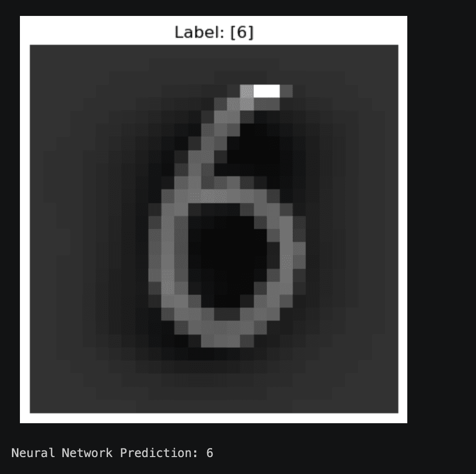
From-scratch neural net correctly identifying a handwritten 6
Scope
14 Models, 4 Domains
- ·K-Nearest Neighbours
- ·Logistic Regression
- ·Naive Bayes
- ·SVM (Linear)
- ·Kernel SVM
- ·Linear Regression
- ·Polynomial Regression
- ·Multiple Linear
- ·Decision Tree
- ·Random Forest
- ·Support Vector (SVR)
- ·K-Means
- ·Hierarchical Clustering
- ·Digit Recognizer (90.84% acc)
- ·Churn Prediction ANN
Highlight
Neural Networks from Scratch
The most technically demanding part of the suite. Two fully-connected neural networks built using only NumPy — no automatic differentiation, no high-level layers. Every gradient is computed manually.
Digit Recognizer — 784 → 30 → 10
Trained on 33,600 handwritten digit images (28×28 px, flattened to 784 inputs). The network learns to classify digits 0–9 with a 10-neuron softmax-style output layer. Achieved 90.84% test accuracy.
Churn Modelling ANN — 12 → 12 → 1
Binary classifier predicting whether a bank customer will churn. Input features include geography, credit score, age, tenure, and balance — one-hot encoded and standardized before training.
The core: backpropagation loop
Each training step runs mini-batch SGD — shuffling the data, splitting into batches, computing gradients via backprop, and updating weights. Every piece of this — the chain rule, the weight updates, the sigmoid derivative — is written by hand.
for epoch in range(self.epochs):
    # Shuffle data each epoch for stochastic behaviour
    indices = np.random.permutation(m)
    X_batches = [X[indices][i:i+batch] for i in range(0, m, batch)]
    y_batches = [y[indices][i:i+batch] for i in range(0, m, batch)]

    for X_mini, y_mini in zip(X_batches, y_batches):
        # Accumulate gradients across the mini-batch
        nabla_w = [np.zeros(w.shape) for w in self.weights]
        nabla_b = [np.zeros(b.shape) for b in self.biases]

        for x, y_true in zip(X_mini, y_mini):
            dw, db = self.backprop(x, y_true)   # compute gradients
            nabla_w = [nw + dw for nw, dw in zip(nabla_w, dw)]
            nabla_b = [nb + db for nb, db in zip(nabla_b, db)]

        # Gradient descent step
        self.weights = [w - lr * nw / batch for w, nw in zip(self.weights, nabla_w)]
        self.biases  = [b - lr * nb / batch for b, nb in zip(self.biases,  nabla_b)]
The network reads a 28×28 pixel image and outputs the correct class label — here, digit 6.
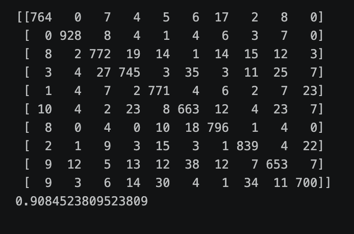
10×10 confusion matrix on the test set. Strong diagonal means the model rarely confuses digits — 90.84% overall accuracy.
Visualizations
Models in Action
Each model was trained on a real dataset and visualized to build intuition for how different algorithms carve up feature space.
Classification — Social Network Ads
Predicting whether a user purchases a product based on Age and Estimated Salary. The two models reveal a key ML insight: the right algorithm depends on your data's shape — linear boundaries work where classes are linearly separable; kernel methods and trees handle the rest.
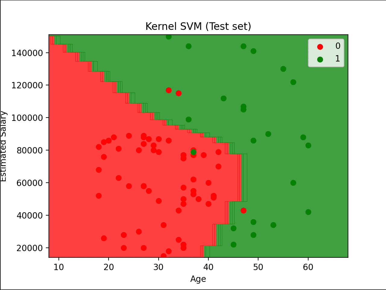
Kernel SVM (RBF) — maps data into a higher-dimensional space, producing a smooth curved boundary that separates the two classes more accurately than a straight line ever could.
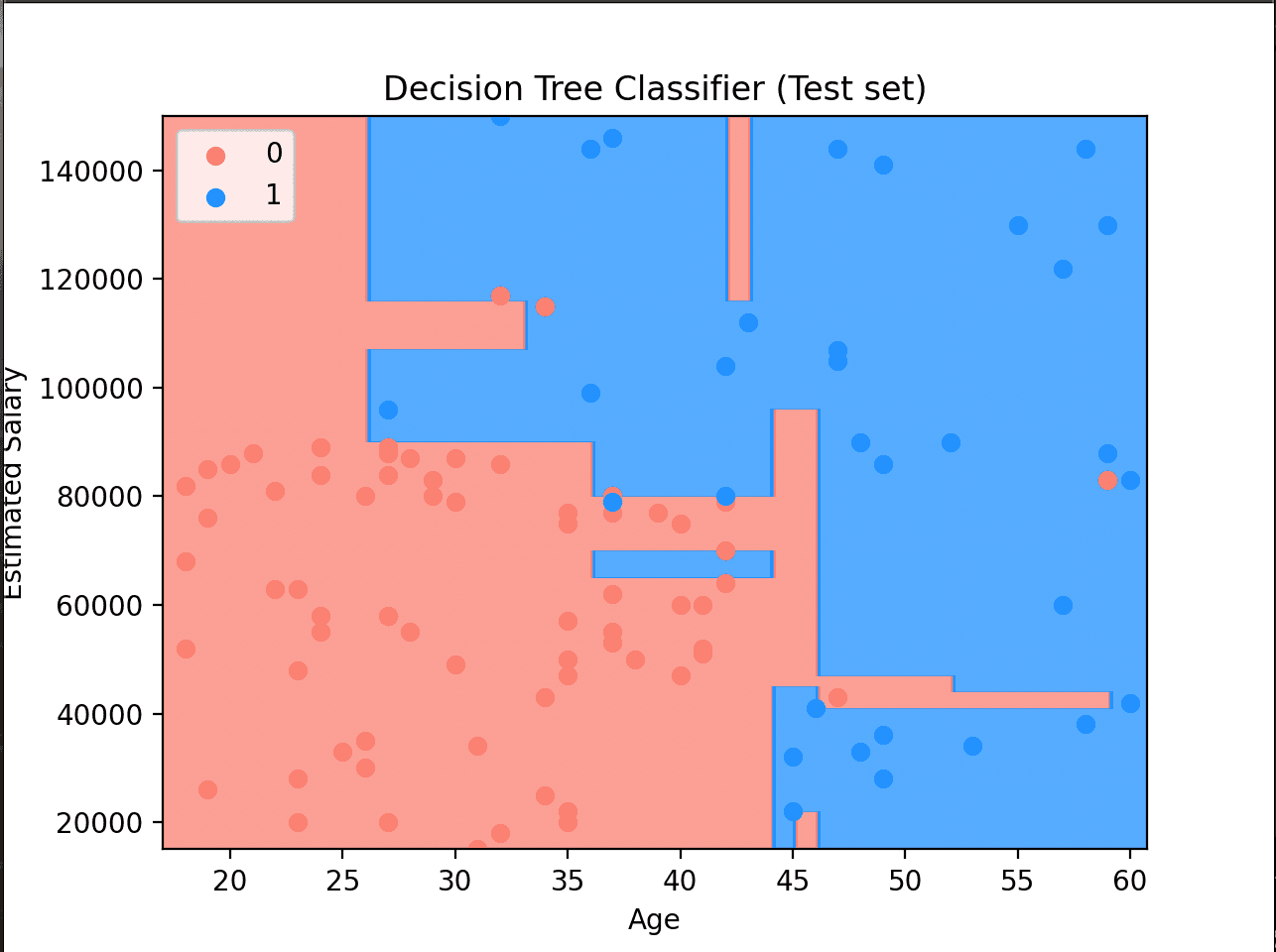
Decision Tree Classifier — the rectangular regions are a signature of axis-aligned splits. Notice the granular pockets where the tree overfit to individual training points.
Clustering — Customer Segmentation
K-Means applied to the Mall Customers dataset, grouping shoppers by Annual Income and Spending Score. The Elbow Method determined k = 5 as the optimal cluster count, producing five clearly defined customer personas.
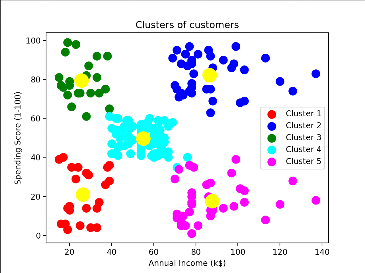
Five distinct customer segments emerge: high income/high spenders (top-right), low income/high spenders (top-left), average everything (center), and two low-spending groups. Yellow dots are cluster centroids.
Regression — Power Plant Energy Output
SVR trained on a power plant dataset to predict energy output (PE) from four environmental variables: Ambient Temperature (AT), Vacuum (V), Ambient Pressure (AP), and Relative Humidity (RH). The kernel fits a non-linear regression curve to each feature.
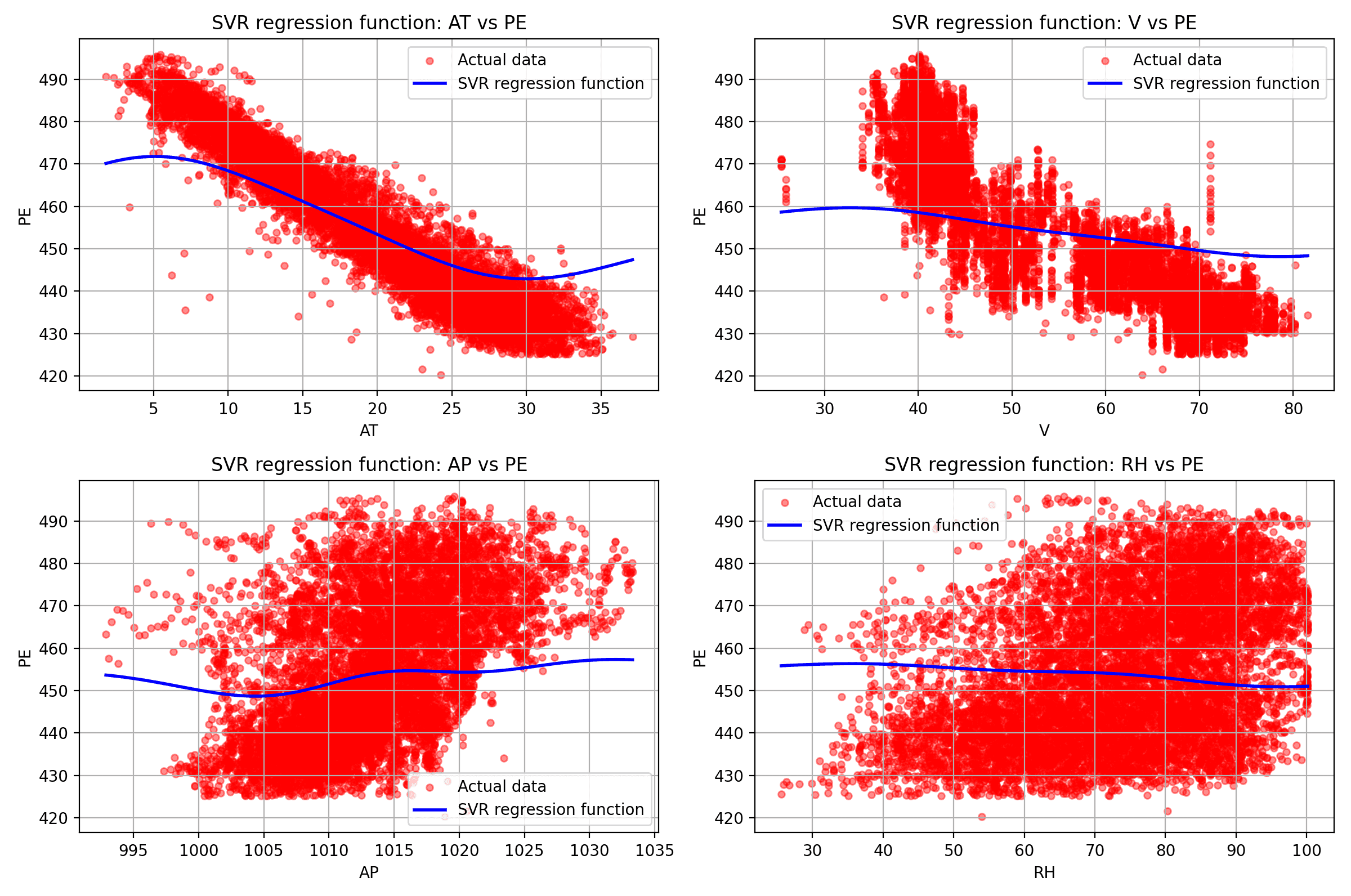
Each panel shows the SVR curve (blue) against actual data points (red). AT has the strongest negative correlation with PE — as the plant runs hotter, output drops.
Takeaways
What This Built
The math behind ML
Writing backprop from scratch made gradient descent and the chain rule concrete — not abstract. You stop treating the network as a black box.
Algorithm intuition
Seeing SVM kernels, decision tree regions, and K-means centroids side-by-side builds real instinct for which tool fits which problem.
Experimental mindset
Each model is a self-contained experiment — different dataset, different objective. The practice of hypothesis → train → visualize → interpret is the same workflow as production ML.